Examples
In the following parts of this chapter we will show you how to use the ARRUS software to communicate with the system in order to:
program the sequence of transmission/reception events (TX/RX) and reconstruction,
acquire raw RF data,
acquire reconstructed B-mode data,
obtain a real-time RF/B-mode/Color Doppler display,
deal with typical issues (time regime, quick switching between sequences, varying tx voltage, etc.).
The source code of the ready-to-run examples can be found in examples directory:
rawRfPwi - for raw RF data acquisition,
bmodePwi - for B-Mode imaging using synthetic aperture & Plane Waves,
bmodeDwi - for B-Mode imaging using synthetic aperture & Diverging Waves,
bmodeLin - for B-Mode imaging using conventional focused line-by-line imaging,
colorPwi - for B-Mode & Color Doppler imaging using synthetic aperture & Plane Waves,
subSequence - for uploading multiple sequences and quick switching between them,
longAcquisition - for long acquisitions and maintaining time regime,
txVoltageLevels - for using different voltage levels for individual tx pulses.
For more information on the parameters of individual functions please refer to section API Reference.
Operations
In ARRUS, you can define and run the operations available for the supported hardware. Transmission/reception (TX/RX) sequences and B-mode image reconstruction are examples of such operations.
TX/RX sequence
To define a TX/RX sequence, you should create an instance of arrus.CustomTxRxSequence class. The name-value input argument pairs allow you to control various aspects of TX/RX.
seq = CustomTxRxSequence('txApertureCenter', 0e-3, ...
                         'txApertureSize',   128, ...
                         'rxApertureCenter', 0e-3, ...
                         'rxApertureSize',   128, ...
                         'txFocus',          inf, ...
                         'txAngle',          (-20:10:20)*pi/180, ...
                         'speedOfSound',     1540, ...
                         'txFrequency',      6.5e6, ...
                         'txNPeriods',       2, ...
                         'txVoltage',        20, ...
                         'rxDepthRange',     50e-3, ...
                         ... % Optional parameters
                         'hwDdcEnable',      true, ...
                         'decimation',       10, ...
                         'nRepetitions',     1, ...
                         'txPri',            400e-6, ...
                         'tgcStart',         14, ...
                         'tgcSlope',         200, ...
                         'txInvert',         false );
The above example shows how to create the CustomTxRxSequence object with a complete set of input parameters. First 11 parameters are obligatory, others are optional.
Interchangeability of parameters
For your convenience:
txApertureCenter [m] can be replaced with txCenterElement [elem],
rxApertureCenter [m] can be replaced with rxCenterElement [elem],
rxDepthRange [m] can be replaced with rxNSamples [samp].
Scalar/vector parameters, sequence length
The following parameters can be scalars or vectors:
txApertureCenter or txCenterElement,
txApertureSize,
rxApertureCenter or rxCenterElement,
txFocus,
txAngle,
txFrequency,
txNPeriods,
txInvert.
If any of them is a vector, then its length determines the number of TXs in the sequence. All the other parameters must be scalars or vectors of the same length. If any parameter is defined as a scalar, then it is assumed to be constant over the whole sequence. If all parameters are scalars, then the sequence contains a single TX/RX.
All the remaining parameters must be scalars, i.e. they are constant for every TX/RX.
Typical TX/RX strategies
To program the typical TX waves:
focused wave: set txFocus to positive finite values [m],
diverging wave: set txFocus to negative finite values [m],
plane wave: set txFocus to inf (as in the code example above).
To program the typical scanning strategies:
phased scanning: set txAngle to a vector of scanning angles [rad] (as in the code example above),
scanning TX aperture: set txApertureCenter [m] or txCenterElement [elem] to a vector of TX aperture positions,
scanning RX aperture: set rxApertureCenter [m] or rxCenterElement [elem] to a vector of RX aperture positions,
Raw data format
The collected raw data format depends on the hwDdcEnable setting:
set hwDdcEnable to false to acquire the original raw RF data,
set hwDdcEnable to true to reduce the data stream, the collected data is in complex IQ format.
For more information, see the documentation of available arrus-api-sequences.
Reconstruction
To define how to perform B-mode image reconstruction, you should create an instance of arrus.Reconstruction class. The name-value input argument pairs allow you to control various aspects of reconstruction.
rec = Reconstruction('xGrid',            (-20:0.10:20)*1e-3, ...
                     'zGrid',            (  0:0.10:50)*1e-3, ...
                     ... % Optional parameters
                     'bmodeRxTangLim',   [-1.0 1.0], ...
                     'rxApod',           hamming(21) ...
                     );
The xGrid and zGrid inputs define the reconstruction grid and thus they are obligatory. Other inputs are optional and allow you to set the size of the dynamic RX aperture (bmodeRxTangLim) and the RX apodization function (rxApod). There are many more optional inputs for setting the raw data filtration, reconstruction mode, Color Doppler, etc.
Running operations in the system
Preparing the system
First, you should create a handle to the system on which you want to perform operations. To communicate with the Us4R system, create an instance of the Us4R class. You will need to indicate a prototxt config file containing the information on the probe, adapter, gains, etc. It is extremly important to make sure that the system configuration agrees with the content of the config file.
us = Us4R('configFile', 'us4r.prototxt');
To run the TX/RX sequence and the reconstruction (optionally), upload them onto the system:
us.upload(seq, rec);
Depending on the sequence length, its upload can take a while. In the use cases that at some point need switching
to another sequence (uploading a new sequence), this upload time can significantly delay the switching. To overcome
this you can upload multiple sequences at once using uploadSequence method:
us.uploadSequence([seq, anotherSeq, yetAnotherSeq]);
The first of the uploaded sequences is selected for execution by default. You can select
any other sequence using its index from the vector of sequences passed to uploadSequence
(indices start from 1):
us.selectSequence(2); % selects anotherSeq
Note that unlike in case of upload, uploadSequence does not assign a reconstruction object
to the uploaded sequences. If you want to do a reconstruction on the data acquired using the selected
sequence, you need to pass the reconstruction object to the system:
us.setReconstruction(rec);
The assignment of the reconstruction to a selected sequence works until the next selectSequence call.
Running the operations
If you only want to run the uploaded/selected operation once (for example, to acquire a single RF frame),
use the run function. It will return the raw RF data (or IQ data if the hwDdcEnable is set to true)
and the reconstructed image data if the reconstruction was uploaded together with the TX/RX sequence.
[rf,img] = us.run;
If you want to run the uploaded operation in a loop e.g. for real-time imaging, use the runLoop function together
with a display-dedicated object. We prepared two classes of display objects: arrus.BModeDisplay and
arrus.DuplexDisplay (for simultaneous display of B-mode and Color Doppler).
display = BModeDisplay(rec, 'dynamicRange', [10 70]);
us.runLoop(@display.isOpen, @display.updateImg);
display = DuplexDisplay(rec, 'dynamicRange',    [10 70], ...
                             'powerThreshold',  20);
us.runLoop(@display.isOpen, @display.updateImg);
Below is an example of image from a wire phantom obtained and displayed with use of the CustomTxRxSequence, Reconstruction, and BModeDisplay objects defined as above.
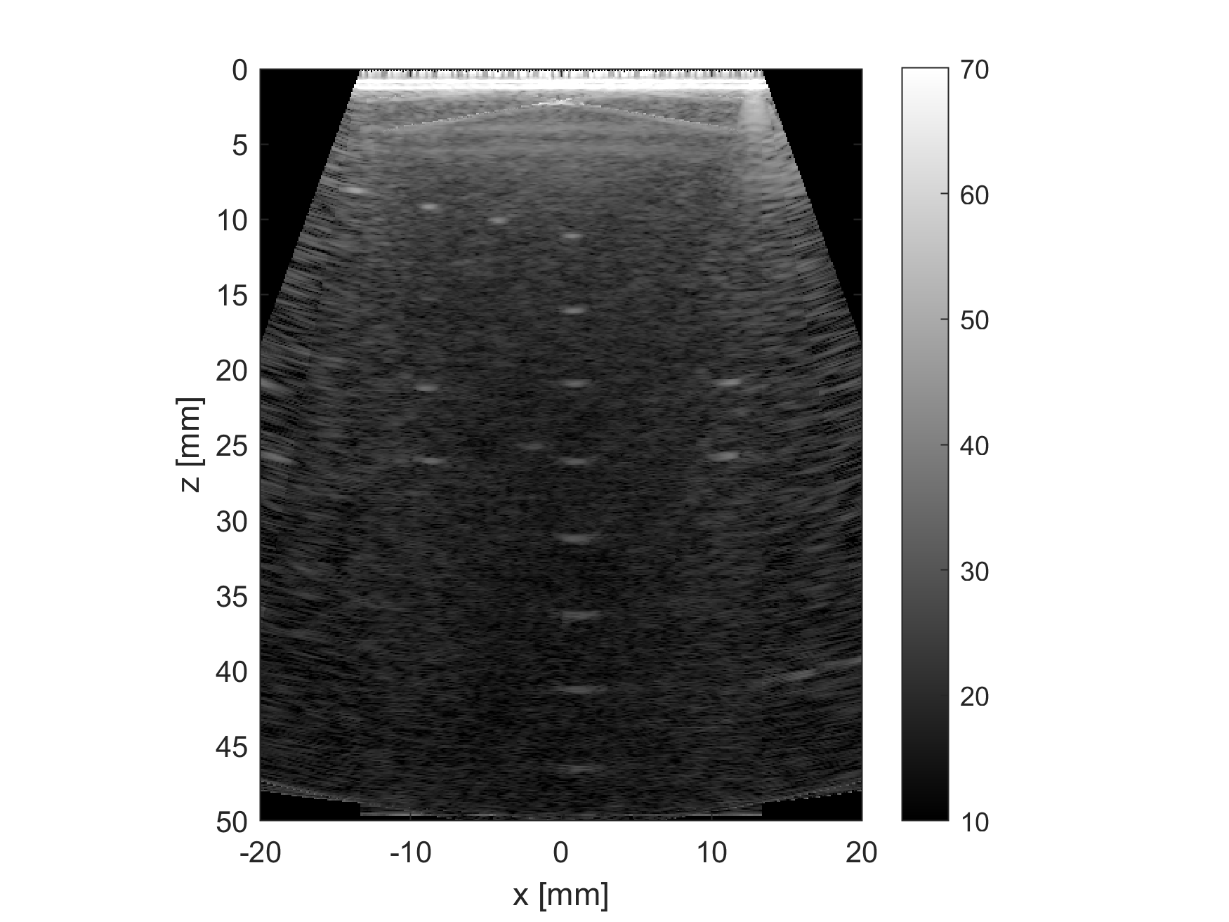
Fig. 2 Image of the ATS549 phantom (wires part) obtained with use of the Plane Wave Imaging.
See the High-level MATLAB scripts docs for more information.
Tips
If you have the object of class Us4R, then you can easily obtain the number of probe elements using getNProbeElem method:
us.getNProbeElem
Specific examples
To present the typical TX/RX issues (except for Color Doppler example), we will use a very simple Reconstruction object with only the reconstruction grid defined (other parameters are assigned default values).
rec = Reconstruction('xGrid', (-30:0.10:30)*1e-3, ...
                     'zGrid', (  0:0.10:40)*1e-3 );
As the reconstruction operates only on the image areas covered by the TX beams, the resulting images will give us insight into the shape, orientation, and position of the TX beams.
Beam formation
The following parameters determine the beam shape, position and orientation:
txFocus [m] - distance between the TX aperture center and the focal point,
txAngle [rad] - angle between the TX beam and the normal to the probe surface at the TX aperture center,
txApertureCenter [m] (or txCenterElement [elem]) - position of the TX aperture center along the probe surface,
txApertureSize [elem] - size of the TX aperture.
Let the following to be our default set of sequence parameters:
seq = CustomTxRxSequence('txApertureCenter', 0e-3, ...
                         'txApertureSize',   48, ...
                         'rxApertureCenter', 0e-3, ...
                         'rxApertureSize',   us.getNProbeElem, ...
                         'txFocus',          inf, ...
                         'txAngle',          0*pi/180, ...
                         'speedOfSound',     1540, ...
                         'txFrequency',      5e6, ...
                         'txNPeriods',       2, ...
                         'txVoltage',        10, ...
                         'rxDepthRange',     50e-3, ...
                         'tgcStart',         14, ...
                         'tgcSlope',         200 );
Now, let us manipulate the parameters determining the TX beam. For various ‘txFocus’ values we can get focused wave (finite positive values), plane wave (infinity), or diverging wave (finite negative values):
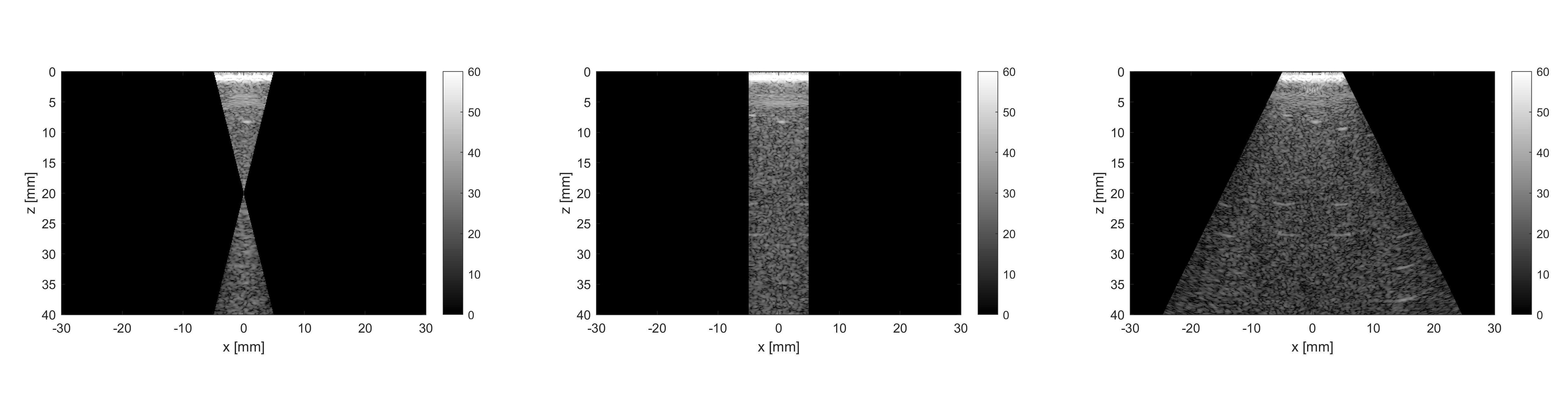
Fig. 3 ‘txFocus’ set to 20e-3 (left), inf (middle), and -10e-3 (right).
When changing the ‘txAngle’ the TX beam axis is angled clockwise (negative values) or counter-clockwise (positive values):
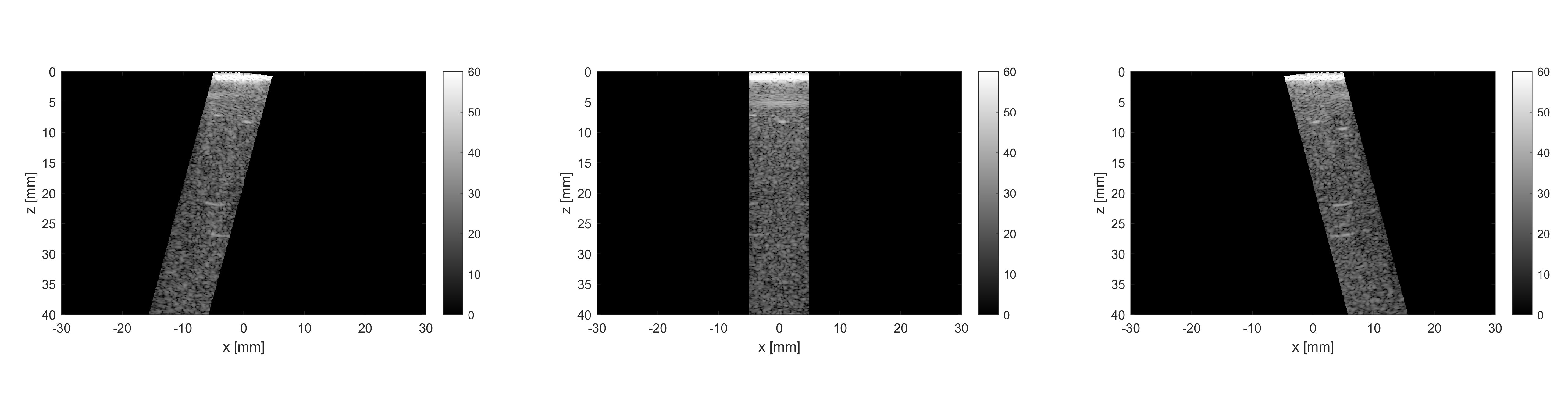
Fig. 4 ‘txAngle’ set to -15*pi/180 (left), 0*pi/180 (middle), and 15*pi/180 (right).
Changing the ‘txApertureCenter’ and ‘txCenterElement’ moves the aperture center along the probe surface.
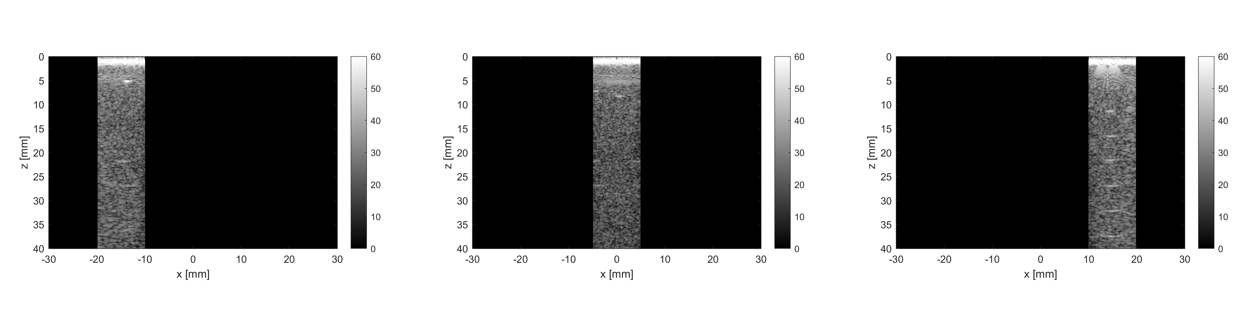
Fig. 5 ‘txApertureCenter’ set to -15e-3 (left), 0e-3 (middle), and 15e-3 (right).
The ‘txApertureSize’ determines how many elements are included in the TX aperture.
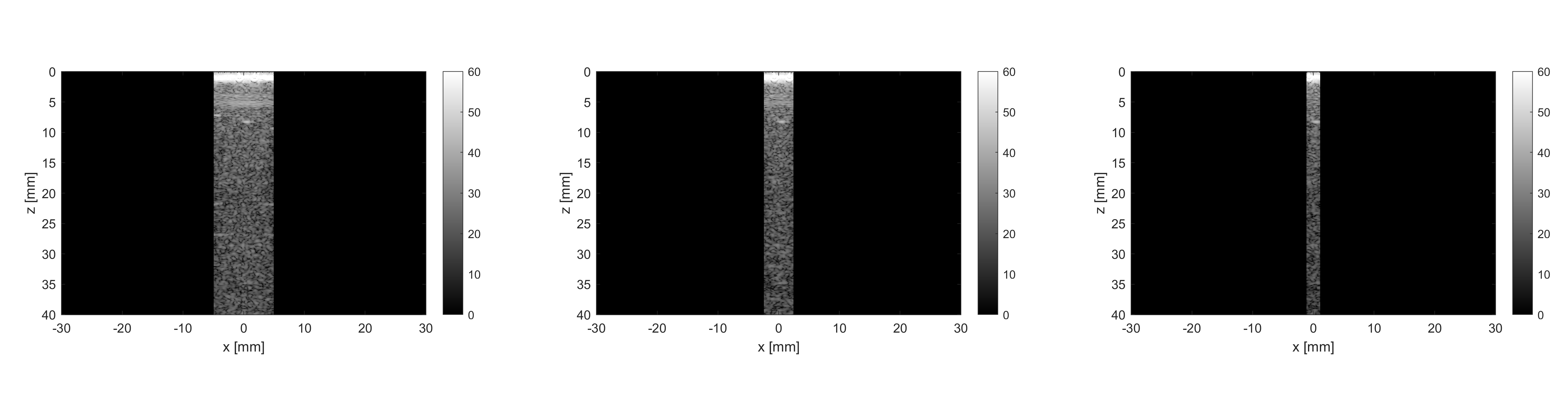
Fig. 6 ‘txApertureSize’ set to 48 (left), 24 (middle), and 12 (right).
In case of a combination of aperture position and size resulting in TX aperture extending beyond the probe, the TX aperture is clipped.
Compounding/scanning strategies
The above examples contained single TXs. It is however typical to use multiple emissions to image wider area (scanning), improve image quality (compounding), etc. The basic scanning strategies will be presented using TX/RX sequences of plane waves emitted from a narrow TX aperture with coarse scanning step, to clearly visualize the process.
Linear scanning
In the linear scanning the TX aperture moves along the probe surface. Usually, the RX aperture does the same. Other parameters are constant:
seq = CustomTxRxSequence(   'txApertureCenter', [-20:10:20]*1e-3, ...
                            'txApertureSize',   32, ...
                            'rxApertureCenter', [-20:10:20]*1e-3, ...
                            'rxApertureSize',   64, ...
                            'txFocus',          inf, ...
                            'txAngle',          0*pi/180, ...
                            % some other parameters
                            );
or
seq = CustomTxRxSequence(   'txCenterElement',  1:32:us.getNProbeElem, ...
                            'txApertureSize',   32, ...
                            'rxCenterElement',  1:32:us.getNProbeElem, ...
                            'rxApertureSize',   64, ...
                            'txFocus',          inf, ...
                            'txAngle',          0*pi/180, ...
                            % some other parameters
                            );
Phased (angular) scanning
In the phased scanning the aperture position is constant, but the TX angle varies.
seq = CustomTxRxSequence(   'txApertureCenter', 0e-3, ...
                            'txApertureSize',   32, ...
                            'rxApertureCenter', 0e-3, ...
                            'rxApertureSize',   64, ...
                            'txFocus',          inf, ...
                            'txAngle',          [-30:15:30]*pi/180, ...
                            % some other parameters
                            );
Custom sequence
Typical imaging schemes use consistent types of waves (e.g. plane wave only) and scanning approaches (e.g. angular scanning only). However, nothing stops us from designing a TX sequence in which all the discussed parameters are varying.
seq = CustomTxRxSequence(   'txApertureCenter', [-20 0 20]*1e-3, ...
                            'txApertureSize',   [32 16 8], ...
                            'txFocus',          [30 inf -5]*1e-3, ...
                            'txAngle',          [-10 0 10]*pi/180, ...
                            % some other parameters
                            );
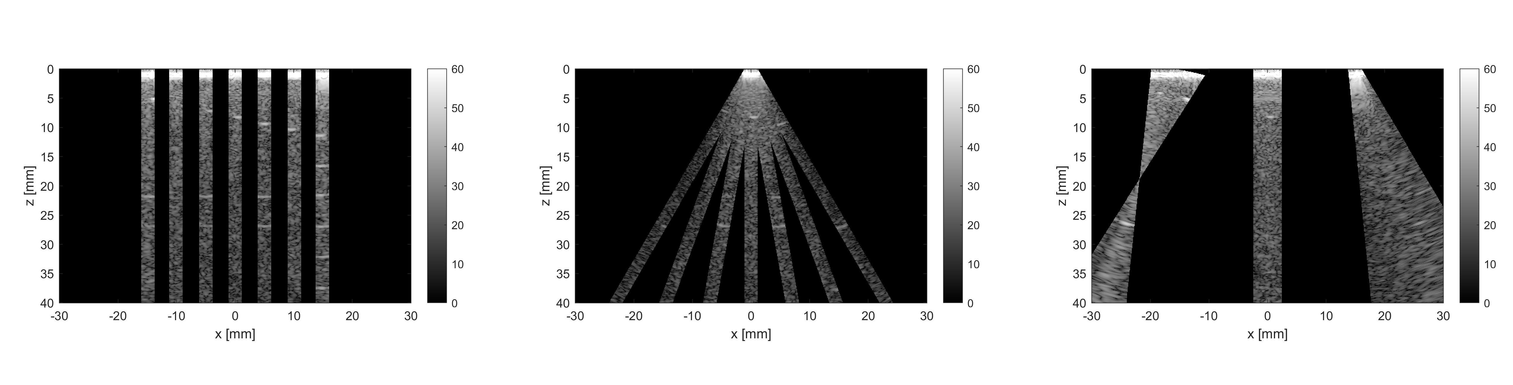
Fig. 7 Example of linear scan (left), angular/phased scan (middle), and custom scan (right).
Probe geometry
What seems clear for linear array, may become not that obvious in the case of convex probe (or any other curved array). To program the TX/RX sequence for a convex probe correctly, one has to remember that:
TX/RX aperture positions are measured along the probe surface, not necessarily along the x-axis (horizontal axis),
TX angles are measured relative to the normal to the head surface at the center of the TX aperture,
TX focuses are measured relative to the center of the TX aperture,
the z-coordinate is adjusted so that z=0 refers to the most withdrawn elements of the probe, which in case of the convex probes are their side elements.
For example, if we set the TX as follows:
seq = CustomTxRxSequence(   'txApertureCenter', -20e-3, ...
                            'txApertureSize',   8, ...
                            'txFocus',          inf, ...
                            'txAngle',          0*pi/180, ...
                            % some other parameters
                            );
then we obtain the following behaviour depending on the geometry of the probe:
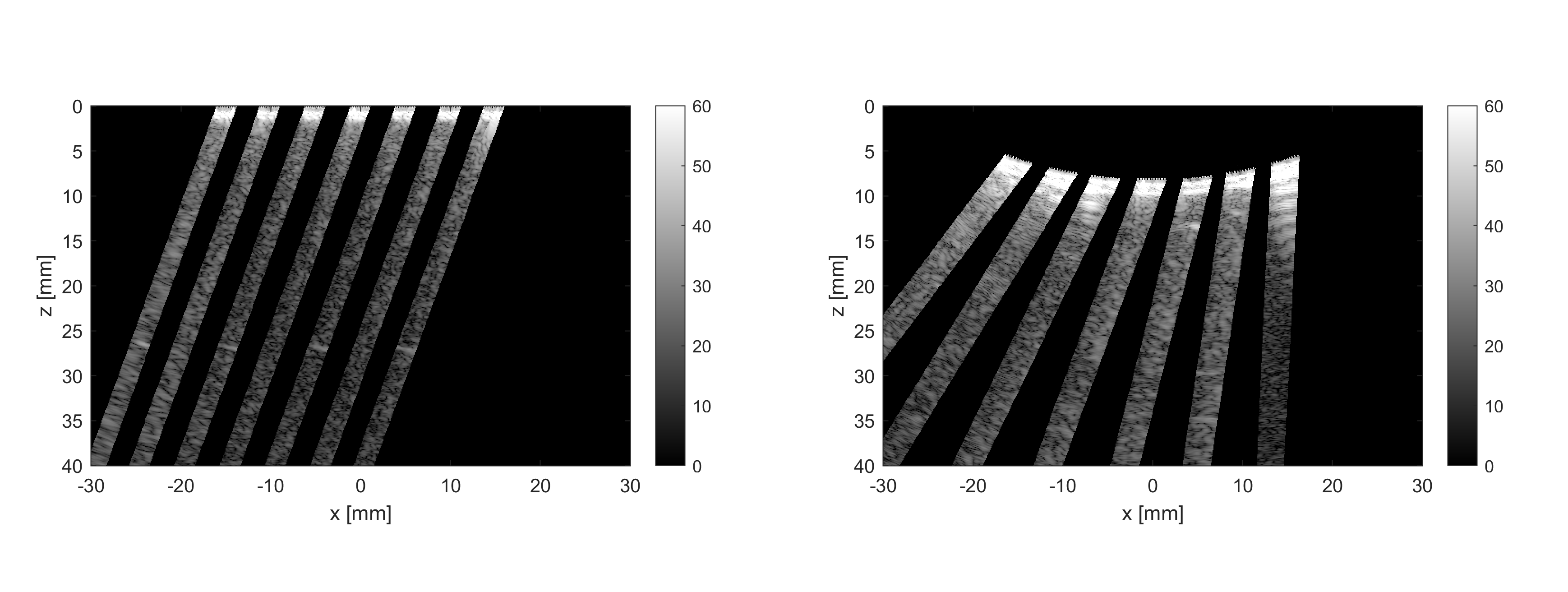
Fig. 8 Example of the probe geometry influence on the programmed TX beams: linear probe (left) and convex probe (right).
Color Doppler
To enable the Color Doppler mode, one has to:
create the TX/RX Sequence that will collect the echoes the same way a given number of times,
create the Reconstruction that will enable and define the Doppler processing.
Below is an example of a sequence that will acquire the data for both: B-mode and Color Doppler. In both modes the sequence utilizes plane waves (‘txFocus’ set to inf) emitted from the whole aperture of the probe, and the echoes are recorded with all the probe elements as well (TX/RX aperture centered at the probe center x=0, aperture size equal to number of probe elements).
In case of B-mode the plane waves will be emitted at 7 different angles for compounding purposes: (-15:5:15)*pi/180.
In case of Color Doppler there will be 32 plane waves, all emitted at 15*pi/180 angle.
seq = CustomTxRxSequence(   'txApertureCenter', 0e-3, ...
                            'txApertureSize',   us.getNProbeElem, ...
                            'rxApertureCenter', 0e-3, ...
                            'rxApertureSize',   us.getNProbeElem, ...
                            'txFocus',          inf, ...
                            'txAngle',          [-15:5:15, 15*ones(1,32)]*pi/180, ...
                            % some other parameters
                            );
The Reconstruction parameters, apart from the reconstruction grid, must contain:
Color Doppler enable flag (‘colorEnable’ set to true),
frame identifiers: frames 1-7 are utilized by B-mode (‘bmodeFrames’ set to 1:7), the following 32 frames are used for Color Doppler (‘colorFrames’ set to 7+(1:32)),
limits of RX tangents for Color Doppler reconstruction (‘colorRxTangLim’). The default is [-0.5 0.5]. It is reasonable to add an offset to make the RX beam angled the same way as the TX beam.
coefficients of a high-pass Wall Clutter Filter (‘wcFilterBCoeff’ and ‘wcFilterACoeff’). Optionally there is a possibility to omit first n output samples of the filter (‘wcFiltInitSize’) to reduce the influence of its transient characteristics.
[wcfB, wcfA] = butter(4,0.2,'high');

rec = Reconstruction(   'xGrid',            (-20:0.10:20)*1e-3, ...
                        'zGrid',            (  0:0.10:30)*1e-3, ...
                        'bmodeFrames',      1:7, ...
                        'colorEnable',      true, ...
                        'colorFrames',      7 + (1:32), ...
                        'colorRxTangLim',   tan(15*pi/180) + [-0.5 0.5], ...
                        'wcFilterBCoeff',   wcfB, ...
                        'wcFilterACoeff',   wcfA, ...
                        'wcFiltInitSize',   8);
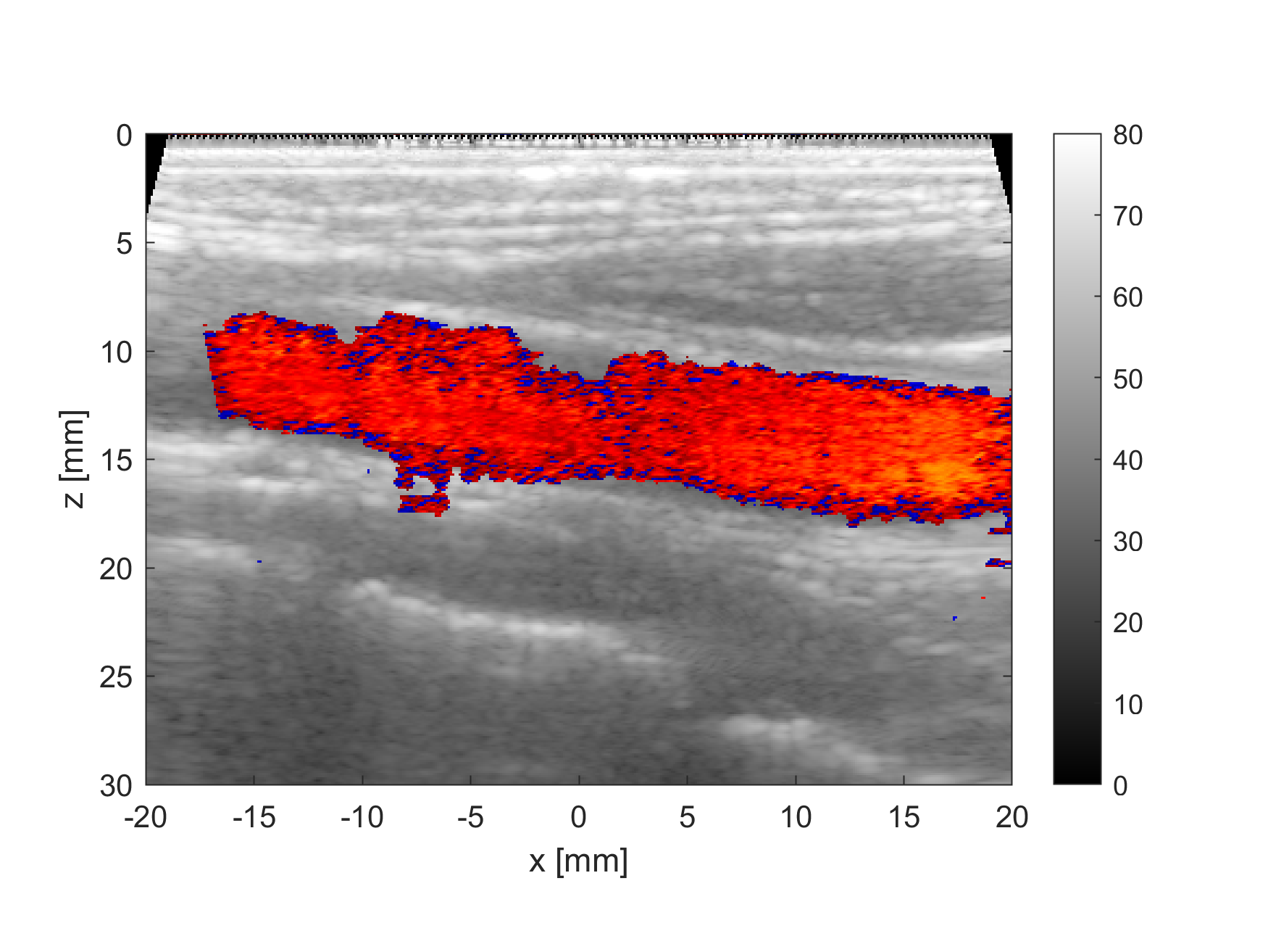
Fig. 9 Color Doppler image of the carotid artery
The source code of the ready-to-run example (colorPwi.m) can be found in the examples directory.
Tips
To obtain good Doppler signal it is suggested to use longer TX pulses (‘txNPeriods’ equal 4 or more).
The Color Doppler scale corresponds to a range from -pi to pi [rad per sample]. To convert it to the Doppler frequencies, one has to know the Pulse Repetition Frequency (PRF) which is given by the formula: PRF = 1/txPri/nFirePerTx. ‘txPri’ is the time between physical emissions and is one of the parameters of the CustomTxRxSequence. nFirePerTx is the number of repeting the emissions needed to acquire the echoes with the programmed RX aperture (e.g. ‘rxApertureSize’ is 192, number of system RX channels is 64, then each TX must be repeated 3 times so that the 64-channel system can acquire 192-channel data).
Quick switching between sequences
Let’s assume that we want a live preview (using sequence seq1 and reconstruction rec1) immediately followed by a collection
of raw data using another sequence (seq2). To avoid time delay due to uploading seq2 after closing the preview, all sequences
should be uploaded together before running the preview, using uploadSequence method. First of the uploaded sequences (seq1)
is selected by default, we just need to set the reconstruction parameters for it using setReconstruction method. To display
the preview, a BModeDisplay object will be used.
Now the system is ready for running live preview using the runLoop method. Immediately after closing the preview window,
seq2 is selected using selectSequence and the raw data is collected using run.
us.uploadSequence([seq1, seq2]);
us.setReconstruction(rec1);

display = BModeDisplay(rec1, 'dynamicRange', [10 70]);
us.runLoop(@display.isOpen, @display.updateImg);

us.selectSequence(2);
rf = us.run;
The source code of the ready-to-run example (subSequence.m) can be found in the examples directory.
Variable TX voltage level
It was mentioned that some parameters of the arrus.CustomTxRxSequence class can be defined as vectors providing values for each TX/RX event individually. Others must be defined as scalars as they are constant for all TX/RX events in a sequence. Well, the txVoltage parameter should be described individually, as it is somewhere between. You can define txVoltage in two ways:
as a scalar v: the voltage range of all TX pulses will be from -v to +v.
as a 2x2 matrix [vn1, vp1; vn2, vp2]: it defines two voltage ranges: first one from -vn1 to +vp1, and the second one from -vn2 to +vp2. Then, for each TX/RX event individually, we can select one of these voltage ranges using the ‘txVoltageId’ parameter. In the below example there is a sequence of plane waves transmissions. The odd ones (with TX angles of: -15,-5,+5,+15 deg) have txVoltageId equal 1, so their TX voltage ranges from -10 to 10 V. For the even ones (TX angle = 0 deg) txVoltageId equals 2, so their amplitude is from -20 to +20 V.
seq = CustomTxRxSequence(   'txFocus',      inf, ...
                            'txAngle',      [-15 0 -5 0 5 0 15 0]*pi/180, ...
                            'txVoltage',    [10 10; 20 20], ...
                            'txVoltageId',  [1 2 1 2 1 2 1 2];
                            % some other parameters
                            );
Note that all elements of the txVoltage matrix must be positive, and the values for the second voltage range must be higher than for the first one.
The source code of the ready-to-run example (txVoltageLevels.m) can be found in the examples directory.
Long acquisitions & time regime
In some applications it may be necessary to collect data at a high and undisturbed rate over a long period of time. There is a limit to the number of TX/RX events in a sequence. If the acquisition is short enough to be covered by a single TX/RX sequence, the time regime is maintained by design. Longer acquisitions may require a repeated executions of the sequence.
Data acquired for a sequence execution are stored in a data buffer, occupying a single buffer element. Transfering the data from the buffer element to the host PC frees the buffer element. If the data are collected faster than they are transferred to the host PC, at some point there will be no free buffer elements for the new data to be stored into (buffer overflow). This, in turn, will result in breaking the time regime. The system can either wait for the buffer to be emptied, or can overwrite the data that were not transferred to the host PC yet (in Matlab this will cause an error).
The example below highlights the parameters of the arrus.CustomTxRxSequence class, that are critical for maintaining the time regime when the sequence is executed multiple times:
workMode: must be set to “SYNC” (optionally “ASYNC” but buffer overflow will throw exceptions).
bufferSize: larger buffer size can help absorb temporary problems with the data transfer to host PC. NOTE: increasing the bufferSize reduces the max. sequence length and increases the upload time.
txPri: it must be adjusted so that it is >= data transfer time.
seq = CustomTxRxSequence(   'workMode',     "SYNC", ...
                            'bufferSize',   8, ...
                            'txPri',        500e-6, ...
                            % some other parameters
                            );
The runLoop method of the arrus.Us4R class offers a cineloop buffer functionality. This buffer is located on the host PC and is limited by its RAM capacity. This buffer should not be confused with the one defined in the arrus.CustomTxRxSequence class, which is located in the Us4R system internal memory. To store the data in the host PC memory, the runLoop method should be called with the following additional arguments:
bufferType: defines the data type to be collected: ‘none’,’raw’,’img’, or ‘all’;
bufferMode: defines acquisition mode: ‘conc’ or ‘subs’, for the data acquisition being concurrent or subsequent to the preview, respectively;
bufferSize: defines the number of acquisition executions to be stored in the buffer;
display = BModeDisplay(rec, 'dynamicRange', [0 80]);

[raw,img,sri] = us.runLoop( @display.isOpen, ...
                            @display.updateImg, ...
                            'bufferType', 'all', ...
                            'bufferMode', 'subs', ...
                            'bufferSize', 1000 ...
                            );
The output of the runLoop method can contain:
raw: raw data (if bufferType was set to ‘raw’ or ‘all’);
img: image data (if bufferType was set to ‘img’ or ‘all’);
sri: sequence repeting intervals for the acquired data;
The source code of the ready-to-run example (longAcquisition.m) can be found in the examples directory.